9/21/16: Friction Forces

Title: Modeling Friction Forces
Purpose: The purpose of this lab is to model static and kinetic friction with various experiments.
Apparatus:
Experiment 1

Experiment 2:

Experiment 3: 

Experiment 4: 

Experiment 5:

Theory: 

Exp. 1: We place a block on a surface and slowly add weights to the end of a string to the point where it just starts to move in order to find the coefficient of static friction. This is repeated with multiple blocks. 

Exp. 2: We attach the block to a force sensor and pull with a constant force to find the coefficient of kinetic friction. This is repeated with multiple blocks. 

Exp. 3: We place the block on the surface and raise it to the angle where it just begins slipping. We use this to find the coefficient of static friction. 

Exp. 4: We attach a motion detector to the top of the incline and place the block so that it will slip down the incline to find the coefficient of kinetic friction. 

Exp. 5: We use the coefficient found in Exp, 4 to find the acceleration of the block when enough weights are placed on it to just get it to move. 

 

Data/Graphs: 

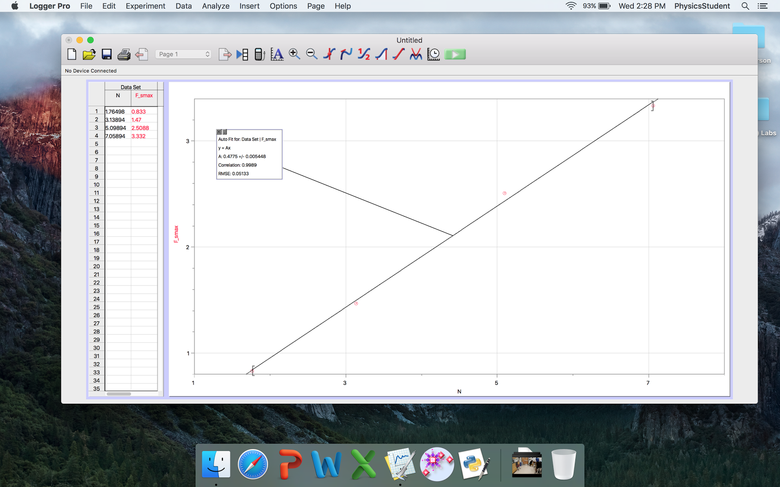
Exp. 1

Exp. 2:

Exp. 3:

Exp. 4:

Exp. 5: 

Analysis: 

Exp. 1: When we plotted the static friction vs. Normal force, we got 0.4775 as a coefficient of static friction. 

Exp. 2: When we graphed the kinetic friction vs Normal force, we got 0.2999 as a coefficient of kinetic friction. 

Exp. 3: The angle at which it started slipping was 26°, and with that we found coefficient of static friction to be 0.488. 

Exp. 4: The angle we measured at was 27°, the acceleration was 2.503 m/s^2, and with that we found the coefficient of kinetic friction to be 0.222. 

Exp. 5: With the coefficient of kinetic friction we found in 4, we used it to find the acceleration of the mass, which was 1.81 m/s^2, slightly different from the calculated 1. 462 m/s^2. 

Conclusion: 

The numbers we calculated theoretically did not vary much from the actual measured results, which meant that we were successful in completing this experiment. Some rooms where errors may have occurred is the when placing the masses to move the block, as the block would move if the weights were placed too fast. Another place where errors could occur was that the place where we placed the block was only a relative position. We did not place the block at the exactly same place every time. 

9/14/16: Air Resistance

Title: Modeling the Fall of an Object Falling with Air Resistance
Purpose:
Determining the relationship between air resistance force and speed.
Predicting terminal velocity of the object with a mathematical model.

Theory:
                                         

The relationship between the air resistance and speed can be modeled with a power law, but we have two unknowns of K and n.

Apparatus:

We dropped coffee filters from a balcony to the ground, starting with 1, and slowly adding up to 5 coffee filters. We captured this motion with LoggerPro and used video capture to be able to plot position and time to find terminal velocity. We plotted the terminal velocity and applied a power curve to find the unknown constants K and n. This gives us a model to be able to predict the air resistance force. We then set up an Excel model similar to the one in Lab 3 for Non-constant Acceleration to predict the terminal velocity to compare the numerical results to the experimental results. 

Data: 

Part 1

Part 2

1CF:

2CF:

3CF:

4CF:

Graphs: 

Explanation/Analysis: 

This is the model we derived from the graph after applying a power fit to the terminal velocities. We did not include the fifth point because it was a stray. It messed up the graph, and the graph looked a lot better when the fifth point was not included. 

Conclusion: 

The answers we arrived at whether numerically or experimentally were pretty close in value. They were precise to the hundredths place. I think some errors that can be accounted for is when we were trying to plot the points for position versus time, as that was a bit time consuming and tedious, and there are a lot of rooms for error at that step. The coffee filters always tend to disappear towards the end of the video, so some of the points were very hard to plot. Regardless, the answers we arrived at were relatively close to each other. 

9/14/16: Trajectories

Title: Trajectories
Purpose:
The purpose of this lab is to use the understanding of projectile motion to predict the impact point of a ball on an inclined board.

Apparatus:

The ball is to be released from a certain height and should theoretically land in the same place each time. 

Theory: 

The theory behind this is to find the launch speed of the ball as it rolls off the ramp and onto the carbon paper. This can be done if the height of the table and the distance of how far it lands is known. After obtaining this information, it can be used further to find how far it would strike a board on an angle, if the angle is known. 

Data: 

This is approximately where the ball landed each time. With this, we found the height of the table to be 94.6cm and the distance x to be 79.6 cm. The angle is 40°. The distance that the ball actually landed on the board at an angle was 70.9cm ± 0.1cm.

Calculations:

Explanation/Analysis: 

The velocity we got was 1.8m/s, and we used that to derive an expression to theoretically calculate "d", which we got to be 0.724m. The experimental value we got for "d" was 70.9 cm ± 0.1 cm, which is fairly close to the answer we got. 

Conclusion: 

The results we got experimentally is fairly close to the answer we got theoretically, meaning that our experiment can be considered a success. There is a -2.07% error, which may be due to an inaccuracies in measuring the heights and lengths of the markings, as it is quite hard to find an exact center to where the ball dropped each time. 

9/12/16: Non-Constant Acceleration

Title: Non-Constant Acceleration
Purpose:
The purpose of this lab is to use Excel to be able to calculate the problem:
A 5000kg elephant on frictionless roller skates is going 25m/s when it gets to the bottom of a hill and arrives on level ground. At that point a 1500kg rocket mounted on the elephant's back generates a constant 8000N thrust opposite the elephant's direction of motion. The mass of the rocket changes with time (due to burning the fuel at a rate of 20kg/s) so that the m(t)=1500kg-20kg/s*t. Find how far the elephant goes before coming to rest.

Theory:
This activity could be done analytically, but it is very complicated and takes a long time.
                                      

                                     

Apparatus/Procedure:
The apparatus of this lab is Microsoft Excel, as all the numerical calculations were done by Excel. Set numbers were listed as constants for initial mass, initial velocity, burning rate, force, and change in time, and there were columns for time, acceleration, average acceleration, change in velocity, velocity, average velocity, change in position, and position.

Data:
For delta t=1
                                     

Delta t=0.1
                                     

Delta t=0.05
                                     

Graphs:
N/A

Analysis:
With a smaller delta t interval, the results are able to be more and more precise. The answer remains the same, but it just gets more and more precise.

Conclusion:
The answer for this, whether analytically or numerically, shows the same answer, meaning that at least the Excel portion of the lab was done correctly. I was able to see that with a smaller t, the answer is more precise, but it does not change the answer in any way.

9/7/16-Free Fall

Title: Free Fall
Purpose:
The purpose of this lab is to examine the validity of the following statement:
In the absence of all other external forces except gravity, a falling body will accelerate at 9.8m/s^2
Apparatus:

                                           

A free falling cylinder is held on the top by an electromagnet. When the magnet releases the object, the spark generator marks periods of the fall of the object at set intervals of 1/60 of a second.
Theory:
With the measured marks, we enter the data in a Excel spreadsheet to graph the data to find velocity and acceleration.

Data:

0
1.8
3.8
6
8.5
11.3
14.3
17.6
21.2
25
29.1
33.4
38.1
43
48.1
53.6
59.3
65.3
71.5
78
84.8
91.9
99.2
106.8
112.4

Graphs: 

Analysis: 

The acceleration is the slope of the velocity vs time graph, which, when converted to the appropriate units, is relatively close to 9.8m/s^2. The slope I got was 9.6m/s^2. In order to find the acceleration with the position vs time graph, I can take the derivative of the equation formed twice to find the acceleration. 

Conclusion: 

The acceleration I got was 9.6 m/s/s, which is relatively close to the "actual" value of the acceleration due to gravity of 9.8 m/s/s. Errors could be made when measuring the differences in the markings, as well as inputing the data into the spreadsheets.

9/7/16: Propagated Uncertainty in Measurements

Title: Propagated Uncertainty in measurements
Purpose:
The purpose of this lab is to make sure how to calculate the propagated error for each measurement of a density.
Apparatus:
                                    

A Vernier Caliper was used to measure accurate lengths of the cylinders, and a balance was used to measure the mass of the cylinders.
Theory:

                                    

The propagated error in the density is found through partial derivatives.
Data:

                                                         

                                   

Calculations:

                                               

                                   

                                    

Analysis:
The density and the propagated error were found through the equations as shown in the Theory section. The process for finding the density and errors for Aluminum were the same as Iron, and therefore only the results are shown.

Conclusion:
The results obtained were reasonable and reliable. The measurements obtained make sense and as a result, the calculations also is reasonable.

8/29/16: Mass/Period Relationship for Inertia Balance

Title: Mass/Period Relationship on an Inertia Balance
Purpose:
The purpose of this lab was to find a relationship between mass and period on an inertial balance. The relationship should be expressed in the form of an equation that is able to predict values accurately.
Apparatus:

The apparatus was an inertial balance clamped to a table. There was tape on one end, which was used to pass through the photogate in order to measure the period. Various masses were placed on the balance to measure the different periods. 

Theory: 

                                     

                                          

If the Mtray measured is correct, the slope should be straight. A straight slope means that the correlation coefficient should be as close to 1 as possible. 

Data: 

                                         

                                         

Calculations/Graph: 

                                         

                                         

                                         

                                         

                                         

Analysis: 

The graphs and data table show that between the masses of 300 and 320 g, the correlation coefficient is the closest to 1, meaning that the slope is a straight line. From that, the values of the slope and y-intercept, which coincides with the unknown values of A and n, are found. From that, we have all of the unknown variables in the equation of the power law. This can be used to determine masses of a variety of objects, as long as we can measure the period of the item. 

Conclusion: 

The relationship found between the mass and the period shows that a greater mass results in a longer period. The calculated mass of the calculator and the actual measured mass of the calculator varies greatly, but the calculated mass of the phone and the actual measured mass of the phone match up quite nicely. I think the error of the calculator may be due to an error in the measuring of the period of the balance, as it may have been not properly centered.